lesscode.net

In Part 1, the first lines of code we saw formed the final step in the construction of the discount curve:

let discs = [ (curveDate, 1.0) ]
            |> bootstrap spotPoints 
            |> bootstrapCash spotDate cashPoints
            |> bootstrapFutures futuresStartDate futuresPoints
            |> bootstrapSwaps spotDate USD swapPoints
            |> Seq.sortBy (fun (qDate, _) -> qDate)

The curve begins with today’s discount factor of 1.0 in a one-element list, which is passed to the bootstrap function along with the spot quotes.

let rec bootstrap quotes discountCurve =
    match quotes with
      quote :: tail -> 
        let newDf = computeDf (List.hd discountCurve) quote
        bootstrap tail (newDf :: discountCurve)
    | [] -> discountCurve

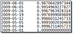
This tail recursion works through the given quotes, computing the discount factor for each based on the previous discount factor in the curve (the details of this we’ll cover in Part 4), and places that new discount factor at the head of a new curve, that is used to continue the recursion. When there are no more quotes, the discount curve is returned, ending the recursion. After bootstrapping the spot quotes, the curve looks like this:

Cash quotes are bootstrapped with respect to the spot discount factor, rather than their previous cash point:

let rec bootstrapCash spotDate quotes discountCurve =
    match quotes with
      quote :: tail -> 
        let spotDf = (spotDate, findDf logarithmic spotDate discountCurve)
        let newDf = computeDf spotDf quote
        bootstrapCash spotDate tail (newDf :: discountCurve)
    | [] -> discountCurve

Here we find the discount factor at the spot date (more about findDf in Part4), tail recurse to compute each cash quote’s corresponding discount factor with respect to the spot discount factor, and prepend that new factor to the discount curve in a similar fashion to the standard bootstrap function. After the cash points are all computed, the curve will be as follows:

Once again, the futures offer a twist, albeit a minor one this time:

let bootstrapFutures futuresStartDate quotes discountCurve =
    match futuresStartDate with
    | Some d ->
        bootstrap (Seq.to_list quotes) 
                  ((d, findDf logarithmic d discountCurve) :: discountCurve)
    | None -> discountCurve

The futures are bootstrapped starting from the beginning of the futures schedule – this is the reason why we calculated futuresStartDate in Part2. For the discount factor at this point, we interpolate using the curve we’ve built thus far. Once that first futures discount point is established, we can place that at the head of a new curve that is subsequently used to bootstrap the futures quotes using the standard approach we employed previously for spot quotes (i.e. each factor is with respect to the last). After the futures, we have this curve:

Note that these aren’t in date order at this point, since we bootstrapped from the futures start date of Jun 17th, but that’s OK for our purposes – it won’t affect the accuracy of the final curve once we sort it chronologically.

Now to the swaps -- this time it’s the swaps that complicate the procedure. With the assumption that the swap quotes are fair market rates (present value zero), we use a root solver (in this case Newton’s method) to find the discount factor of each swap, pricing them using the curve we’ve built thus far:

let rec bootstrapSwaps spotDate calendar swapQuotes discountCurve =
    match swapQuotes with
      (qDate, qQuote) :: tail ->
        // build the schedule for this swap                
        let swapDates = schedule semiAnnual { startDate = spotDate; endDate = qDate }
        let rolledSwapDates = Seq.map (fun (d:Date) -> roll RollRule.Following calendar d) 
                                      swapDates
        let swapPeriods = Seq.to_list (Seq.map (fun (s, e) -> { startDate = s; endDate = e }) 
                                      (Seq.pairwise rolledSwapDates))
        
        // solve
        let accuracy = 1e-12
        let spotFactor = findDf logarithmic spotDate discountCurve
        let f = computeSwapDf dayCount spotDate (qDate, qQuote) discountCurve swapPeriods 
        let newDf = solveNewton f accuracy spotFactor                   

        bootstrapSwaps spotDate calendar tail ((qDate, newDf) :: discountCurve)
    | [] -> discountCurve

For each swap we build a semi-annual schedule from spot to swap maturity using the schedule function, which recursively builds a sequence of dates six months apart:

let rec schedule frequency period =
    seq {
        yield period.startDate
        let next = frequency period.startDate
        if (next <= period.endDate) then
            yield! schedule frequency { startDate = next; endDate = period.endDate }
    }

Where frequency (in this case semiAnnual) is a function in its own right, that does – guess what?

let semiAnnual (from:Date) = from.AddMonths(6)

Each of the schedule dates in the sequence is then rolled according to the Following rolling rule, and then taken pairwise to generate a schedule of unbroken start and end dates for each period. This schedule is used to calculate both the discount factor and the first derivative of each swap quote, which in turn feed Newton’s method along with our desired accuracy of twelve decimals. Each result is placed at the head of our growing discount curve which will be used to compute the next swap discount factor. In the end our complete curve looks like this:

In Part 4, we’ll dive into to (relatively simple) math functions that underpin the bootstrapping calculations.